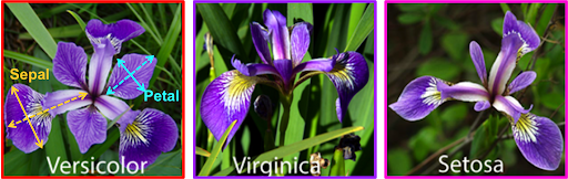
2. Iris의 세 가지 품종, 분류해볼 수 있겠어요?

학습 목표

• scikit-learn에 내장되어 있는 예제 데이터셋의 종류를 알고 활용할 수 있다.
• scikit-learn에 내장되어 있는 분류 모델들을 학습시키고 예측해 볼 수 있다.
• 모델의 성능을 평가하는 지표의 종류에 대해 이해하고, 활용 및 확인해 볼 수 있다.
• Decision Tree, SGD, RandomForest, 로지스틱 회귀 모델을 활용해서 간단하게 학습 및 예측해 볼 수 있다.
• 데이터셋을 사용해서 스스로 분류 기초 실습을 진행할 수 있다.

1. 붓꽃 분류 문제

(1) 어떤 데이터를 사용할 것인가?

붓꽃 데이터는 머신러닝에서 많이 사용되는 라이브러리 중 하나인 사이킷런(scikit-learn)에 내장되어 있는 데이터이다.

사이킷런 데이터셋

사이킷런에서는 두 가지 데이터셋을 제공한다

• 비교적 간단하고 작은 데이터셋인 Toy datasets
• 복잡하고 현실 세계를 반영한 Real world datasets

(2) 데이터 준비

# datasets 불러오기
from sklearn.datasets import load_iris

iris = load_iris()
print(type(dir(iris))) # dir()는 객체가 어떤 변수와 메서드를 가지고 있는지 나열함

# 메서드 확인
iris.keys()

iris_data = iris.data # iris.method 로 해당 메소드를 불러올 수 있다.

# shape는 배열의 형상 정보를 출력
print(iris_data.shape)

# 각 label의 이름
iris.target_names

# 데이터셋에 대한 설명
print(iris.DESCR)

# 각 feature의 이름
iris.feature_names

# datasets의 저장된 경로
iris.filename

# pandas 불러오기
import pandas as pd

print(pd.__version__) # pandas version 확인

# DataFreame 자료형으로 변환하기
iris_df = pd.DataFrame(data=iris_data, columns=iris.feature_names)
iris_df["label"] = iris.target

(3) train, test 데이터 분리

# train_test_split 함수를 이용하여 train set과 test set으로 나누기
from sklearn.model_selection import train_test_split

x_train, x_test, y_train, y_test = train_test_split(iris_data,
                                                    iris_label,
                                                    test_size=0.2,
                                                    random_state=7)

print(f'x_train 개수: {len(x_train)}, x_test 개수: {len(x_test)}')

(4) 모델 학습 및 예측

• 사용할 모델
  • Decision Tree (의사 결정 트리)
  • Random Forest
  • Support Vector Machine (SVM)
  • Stochastic Gradient Descent (SGD)
  • Logisitic Regression (로지스틱 회귀)

# Decision Tree 사용하기
from sklearn.tree import DecisionTreeClassifier

decision_tree = DecisionTreeClassifier(random_state=32)

print(decision_tree._estimator_type) # decision_tree 의 type 확인

decision_tree.fit(x_train, y_train)
y_pred = decision_tree.predict(x_test)

print(classification_report(y_test, y_pred))

# Random Forest
from sklearn.ensemble import RandomForestClassifier

random_forest = RandomForestClassifier(random_state=32)
random_forest.fit(x_train, y_train)
y_pred = random_forest.predict(x_test)

print(classification_report(y_test, y_pred))

# Support Vector Machine (SVM)
from sklearn import svm

svm_model = svm.SVC()
svm_model.fit(x_train, y_train)
y_pred = svm_model.predict(x_test)

print(classification_report(y_test, y_pred))

# Stochastic Gradient Desecnt(SGD)
from sklearn.linear_model import SGDClassifier

sgd_model = SGDClassifier()
sgd_model.fit(x_train, y_train)
y_pred = sgd_model.predict(x_test)

print(classification_report(y_test, y_pred))

# Logisitc Regression
from sklearn.linear_model import LogisticRegression

logistic_model = LogisticRegression(max_iter=200)
logistic_model.fit(x_train, y_train)
y_pred = logistic_model.predict(x_test)

print(classification_report(y_test, y_pred))

단순히 라이브러리에서 데이터와 함수를 불러오는 것 만으로도 쉽게 머신러닝 모델을 만들 수 있다.

2. 데이터의 불균형으로 인한 정확도의 오류

(1) 믿을 수 있는 데이터인가?

사이킷런 라이브러리를 이용하여 만든 머신러닝 모델들은 모두 괜찮은 정확도를 보여주었다. 그러나 이 데이터가 정말로 믿을 수 있는, 유효한 데이터인가?

예를 들어, test set의 정답 레이블이 [0, 0, 0, 0, 1, 0, 0, 0, 0, 0] 이라고 할 때, 모델의 학습이 잘못되어서 제대로 판단할 수 없지만 출력값은 0으로 처리한다고 하면 이 모델의 정확도는 90%라고 할 수 있을까?

이것을 판단하기 위해서 Confusion Matrix(혼동 행렬)에 대해 알아보자.

(2) Confusion Matrix

혼동 행렬은 주로 알고리즘 분류 알고리즘의 성능을 시각화 할 수 있는 표이다. 따라서 해당 모델이 True를 얼만큼 True라고 판단했는지, False를 얼만큼 False라고 판단했는지 쉽게 확인할 수 있다.

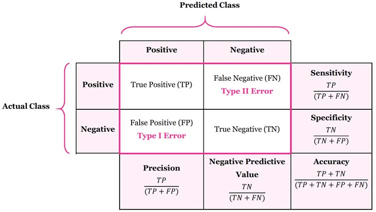
알고리즘의 성능을 판단할 때에는 어디에 적용되는 알고리즘인가를 먼저 생각한 후에 판단할 수 있다. 예를 들어, 스팸 메일을 분류한다고 할 때, 스팸 메일은 정상 메일로 분류되어도 괜찮지만, 정상 메일은 스팸 메일로 분류되어서는 안된다. 또는 환자의 암을 진단할 때, 음성을 양성으로 진단하는 것 보다 양성을 음성으로 진단하는 것은 큰 문제를 일으킬 수 있다. 따라서 상황에 맞는 지표를 활용할 줄 알아야 한다.

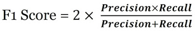
추가로, F1 Score 라는 지표도 있는데, 해당 지표는 Precision과 Recall(Sensitivity)의 조화평균이며, Precision과 Recall이 얼마나 균형을 이루는지 쉽게 알 수 있는 지표이다.

3. 다른 모델 분류해보기

이번에는 사이킷런에 있는 다른 데이터셋을 공부한 모델을 이용하여 학습시켜보고 결과를 예측해보자.

(1) digits 분류하기

# (1) 필요한 모듈 import
from sklearn.datasets import load_digits
from sklearn.model_selection import train_test_split
from sklearn.tree import DecisionTreeClassifier
from sklearn.ensemble import RandomForestClassifier
from sklearn import svm
from sklearn.linear_model import SGDClassifier
from sklearn.linear_model import LogisticRegression
from sklearn.metrics import classification_report
from sklearn.metrics import recall_score

# (2) 데이터 준비
digits = load_digits()
digits_data = digits.data
digits_label = digits.target

# (3) train, test 데이터 분리
x_train, x_test, y_train, y_test = train_test_split(digits_data, 
                                                    digits_label, 
                                                    test_size=0.2, 
                                                    random_state=7)

# 정규화
x_train_norm, x_test_norm = x_train / np.max(x_train), x_test / np.max(x_test)

# (4) 모델 학습 및 예측
# Decision Tree
decision_tree = DecisionTreeClassifier(random_state=32)
decision_tree.fit(x_train_norm, y_train)
decision_tree_y_pred = decision_tree.predict(x_test_norm)
print(classification_report(y_test, decision_tree_y_pred))

# RandomForest
random_forest = RandomForestClassifier(random_state=32)
random_forest.fit(x_train_norm, y_train)
random_forest_y_pred = random_forest.predict(x_test_norm)
print(classification_report(y_test, random_forest_y_pred))

# SVM
svm_model = svm.SVC()
svm_model.fit(x_train_norm, y_train)
svm_y_pred = svm_model.predict(x_test_norm)
print(classification_report(y_test, svm_y_pred))

# SGD
sgd_model = SGDClassifier()
sgd_model.fit(x_train_norm, y_train)
sgd_y_pred = sgd_model.predict(x_test_norm)
print(classification_report(y_test, sgd_y_pred))

# Logistic Regression
logistic_model = LogisticRegression(max_iter=256)
logistic_model.fit(x_train_norm, y_train)
logistic_y_pred = logistic_model.predict(x_test_norm)
print(classification_report(y_test, logistic_y_pred))

• 예상 결과

  이미지 파일은 2차원 배열이기 때문에 SVM을 이용하여 한 차원 늘려서 Date를 Clustering 한다면 가장 좋은 결과를 얻을 것이다.

  숫자 인식은 해당 숫자를 정확한 숫자로 인식한 결과값만이 의미가 있다고 생각하기 때문에 Recall 값을 비교하여 성능을 판단할 것이다.

• 실제 결과

    print('Decision Tree       : {}'.format(recall_score(y_test, decision_tree_y_pred, average='weighted')))
    print('Random Forest       : {}'.format(recall_score(y_test, random_forest_y_pred, average='weighted')))
    print('SVM                 : {}'.format(recall_score(y_test, svm_y_pred, average='weighted')))
    print('SGD                 : {}'.format(recall_score(y_test, sgd_y_pred, average='weighted')))
    print('Logistic Regression : {}'.format(recall_score(y_test, logistic_y_pred, average='weighted')))
  
    Decision Tree       : 0.8555555555555555
    Random Forest       : 0.9638888888888889
    SVM                 : 0.9888888888888889
    SGD                 : 0.9472222222222222
    Logistic Regression : 0.9611111111111111

  예상한 것과 마찬가지로 SVM이 가장 좋은 성능을 나타내는 것으로 볼 수 있다.

(2) wine 분류하기

# (1) 필요한 모듈 import
from sklearn.datasets import load_wine
from sklearn.model_selection import train_test_split
from sklearn.tree import DecisionTreeClassifier
from sklearn.ensemble import RandomForestClassifier
from sklearn import svm
from sklearn.linear_model import SGDClassifier
from sklearn.linear_model import LogisticRegression
from sklearn.metrics import classification_report
from sklearn.metrics import recall_score

# (2) 데이터 준비
wines = load_wine()
wines_data = wines.data
wines_label = wines.target

# (3) train, test 데이터 분리
x_train, x_test, y_train, y_test = train_test_split(wines_data, 
                                                    wines_label, 
                                                    test_size=0.2, 
                                                    random_state=7)

# (4) 모델 학습 및 예측
# Decision Tree
decision_tree = DecisionTreeClassifier(random_state=32)
decision_tree.fit(x_train, y_train)
decision_tree_y_pred = decision_tree.predict(x_test)
print(classification_report(y_test, decision_tree_y_pred))

# RandomForest
random_forest = RandomForestClassifier(random_state=32)
random_forest.fit(x_train, y_train)
random_forest_y_pred = random_forest.predict(x_test)
print(classification_report(y_test, random_forest_y_pred))

# SVM
svm_model = svm.SVC()
svm_model.fit(x_train, y_train)
svm_y_pred = svm_model.predict(x_test)
print(classification_report(y_test, svm_y_pred))

# SGD
sgd_model = SGDClassifier()
sgd_model.fit(x_train, y_train)
sgd_y_pred = sgd_model.predict(x_test)
print(classification_report(y_test, sgd_y_pred))

# Logistic Regression
logistic_model = LogisticRegression(max_iter=4096)
logistic_model.fit(x_train, y_train)
logistic_y_pred = logistic_model.predict(x_test)
print(classification_report(y_test, logistic_y_pred))

• 예상 결과

  와인은 여러가지 특징에 따라 종류가 나뉘어지기 때문에 Decision Tree 또는 Random Forest가 가장 좋은 성능을 나타낼 것으로 예상된다. 아무래도 발전된 모델인 Random Forest 쪽이 더 좋은 결과가 나올 것 같다.

  와인도 숫자와 마찬가지로 정확하게 분류한 값만이 의미가 있다고 생각하기 때문에 Recall 값을 비교하여 성능을 판단할 것이다.

• 실제 결과

    print('Decision Tree       : {}'.format(recall_score(y_test, decision_tree_y_pred, average='weighted')))
    print('Random Forest       : {}'.format(recall_score(y_test, random_forest_y_pred, average='weighted')))
    print('SVM                 : {}'.format(recall_score(y_test, svm_y_pred, average='weighted')))
    print('SGD                 : {}'.format(recall_score(y_test, sgd_y_pred, average='weighted')))
    print('Logistic Regression : {}'.format(recall_score(y_test, logistic_y_pred, average='weighted')))
  
    Decision Tree       : 0.9444444444444444
    Random Forest       : 1.0
    SVM                 : 0.6111111111111112
    SGD                 : 0.5277777777777778
    Logistic Regression : 0.9722222222222222

  예상한 것과 마찬가지로 Random Forest가 가장 우수한 성능을 보여준다. 아무래도 Feature에 따라 와인의 종류가 확실하게 구분될 수 있기 때문인 것 같다.

  (3) breast cancer 분류하기

  ---

    # (1) 필요한 모듈 import
    from sklearn.datasets import load_breast_cancer
    from sklearn.model_selection import train_test_split
    from sklearn.tree import DecisionTreeClassifier
    from sklearn.ensemble import RandomForestClassifier
    from sklearn import svm
    from sklearn.linear_model import SGDClassifier
    from sklearn.linear_model import LogisticRegression
    from sklearn.metrics import classification_report
    from sklearn.metrics import recall_score
  
    # (2) 데이터 준비
    breast_cancer = load_breast_cancer()
    breast_cancer_data = breast_cancer.data
    breast_cancer_label = breast_cancer.target
  
    # (3) train, test 데이터 분리
    x_train, x_test, y_train, y_test = train_test_split(breast_cancer_data, 
                                                        breast_cancer_label, 
                                                        test_size=0.2, 
                                                        random_state=7)
  
    # (4) 모델 학습 및 예측
    # Decision Tree
    decision_tree = DecisionTreeClassifier(random_state=32)
    decision_tree.fit(x_train, y_train)
    decision_tree_y_pred = decision_tree.predict(x_test)
    print(classification_report(y_test, decision_tree_y_pred))
  
    # RandomForest
    random_forest = RandomForestClassifier(random_state=32)
    random_forest.fit(x_train, y_train)
    random_forest_y_pred = random_forest.predict(x_test)
    print(classification_report(y_test, random_forest_y_pred))
  
    # SVM
    svm_model = svm.SVC()
    svm_model.fit(x_train, y_train)
    svm_y_pred = svm_model.predict(x_test)
    print(classification_report(y_test, svm_y_pred))
  
    # SGD
    sgd_model = SGDClassifier()
    sgd_model.fit(x_train, y_train)
    sgd_y_pred = sgd_model.predict(x_test)
    print(classification_report(y_test, sgd_y_pred))
  
    # Logistic Regression
    logistic_model = LogisticRegression(max_iter=4096)
    logistic_model.fit(x_train, y_train)
    logistic_y_pred = logistic_model.predict(x_test)
    print(classification_report(y_test, logistic_y_pred))

  • 예상 결과

    유방암의 경우에는 feature의 갯수가 많아서 Decision Tree 또는 Random Forest가 우수한 성능을 나타낼 것으로 예상된다. 또한 양성/음성 이진 분류 문제이기 때문에 Logistic Regression도 좋은 성능을 나타낼 것으로 예상된다.

    유방암은 양성을 양성으로 판단한 값이 중요하지만, 음성을 음성으로 판단한 값도 중요하기 때문에 accuracy를 기준으로 성능을 판단할 것이다.

  • 실제 결과

      print('Decision Tree       : {}'.format(recall_score(y_test, decision_tree_y_pred, average='weighted')))
      print('Random Forest       : {}'.format(recall_score(y_test, random_forest_y_pred, average='weighted')))
      print('SVM                 : {}'.format(recall_score(y_test, svm_y_pred, average='weighted')))
      print('SGD                 : {}'.format(recall_score(y_test, sgd_y_pred, average='weighted')))
      print('Logistic Regression : {}'.format(recall_score(y_test, logistic_y_pred, average='weighted')))
    
      Decision Tree       : 0.9122807017543859
      Random Forest       : 1.0
      SVM                 : 0.9035087719298246
      SGD                 : 0.9035087719298246
      Logistic Regression : 0.9473684210526315

    예상한 것과 마찬가지로 Random Forest가 가장 우수한 성능을 보여준다. 아무래도 Feature의 종류가 많아 이진 분류 문제에 정확도를 더 높여줄 수 있었던 것 같다. 물론 Logisitc Regression도 충분히 좋은 성능을 보여주었다.

이번엔 머신러닝의 가장 기본적인 모델들에 대해서 학습하였다. 라이브러리를 이용해서 직접 간단한 학습 모델도 구현해보면서 각 모델들에 대한 이해력이 높아졌다. 모델의 성능을 나타낼 때, 정확도가 중요한 것은 알고 있었지만 성능을 나타내는 지표에 이렇게 많은 지표들이 있다는 것은 처음 알게되었다. 생각해보면 당연한 사실이어서 개념이 어렵지는 않았다. 앞으로도 이 정도의 학습량이라면 충분히 문제없이 따라갈 수 있을 것 같다.

get_next_line

Prototype

int get_next_line(int fd, char **line);

Turn in files

• get_next_line.c
• get_next_line_utils.c
• get_next_line.h

Parameters

1. file descriptor for reading
2. the value of what has been read

Return value

• 1 : A line has been read
• 0 : EOF has been reached
• -1 : An error happend

External functs.

• read, malloc, free

Description

• Write a function which returns a line read from a file descriptor, without the newline

선행지식

1. File descriptor 관련

• https://docs.oracle.com/cd/E19476-01/821-0505/file-descriptor-requirements.html
• https://lowlevel.tistory.com/3

2. Read 함수

ssize_t read(int fd, void *buf, size_t count);

Description

• fd에서 count 만큼 읽어 buf에 저장한다.

Return value

• 읽은 count 만큼 return. 에러가 발생했을 시 -1을 return한다.

3. Static variable

• 지역변수와 전역변수의 성질을 동시에 가지고 있는 변수. 프로그램이 종료될 때 까지 메모리에 남아있기 때문에 gnl 함수가 다시 호출되었을 때 첫 번째 line이 아닌 두 번째 line을 읽을 수 있도록 할 수 있다. 함수 내에서만 사용이 가능하지만 전역변수처럼 사용이 가능하다.
• https://blog.naver.com/ddck1321/221865835857

목표

• get_next_line 함수를 호출하면 EOF 전 까지 file descriptor에서 한 번에 한 줄을 읽을 수 있어야 한다.
• file로 부터 읽는 경우와 standard input에서도 작동할 수 있어야 한다.
• 컴파일 시에 -D BUFFER_SIZE=XX flag를 사용하여 BUFFER_SIZE를 임의로 변경할 수 있으며 정의되지 않을 땐 적절한 값을 사용해야 한다.
• BUFFER_SIZE가 매우 클 때 (10000000) 일 때에도 정상적으로 작동해야 한다.
• Static variable을 하나만 사용하여 함수 구현하기.

구현 방법

1. fd에서 적절한 BUFFER_SIZE만큼 읽어 buf에 저장한다.
2. buf를 static 변수에 backup 해둔다.
3. static 변수에 개행이 있는지 확인 후 없다면 다시 읽는다.
4. static 변수에 개행이 있다면 개행 전 까지 line에 저장하고, 개행 후로는 다시 static변수에 저장한다.

• 처음에 get_next_line 함수를 완성하고 테스트를 돌려봤을 때 첫 한 줄만 출력이 되고 그 다음줄은 출력이 되지 않았다. 원인을 찾아보니 get_next_line 함수를 2회째 호출할 때 부터 backup 변수에 남아있어야 할 문자열이 사라져 있는 것이었다.
• get_next_line 함수에서 find_ret_value함수로 backup 값을 넘겨줄 때, static variable은 해당 함수 안에서만 값을 변경할 수 있기 때문에 다른 함수에서도 값을 변경하기 위해서는 &연산자를 이용하여 주소값을 넘겨주어야 했다.
• main을 만들어서 테스트 결과, subject에서 원하는 결과와 같이 출력은 되었으나, 다른 사람들이 만들어 놓은 테스트를 돌려본 결과, 일부 BUFFER_SIZE와 매우 큰 BUFFER_SIZE에서 오류가 발생하였다.
• BUFFER_SIZE를 정적으로 할당할 경우 매우 큰 수의 경우에는 할당이 불가하여 segfault 오류가 발생할 수 있으므로 동적할당으로 수정하였다.

get_next_line은 과제 이후에도 다른 프로젝트에서 계속 사용하기 때문에 잘 만들어두는 것이 좋다. 그렇지 않으면 나중에 다른 과제를 할 때 get_next_line을 고치고 있어야 할 지도 모르니까... 지금 내가 그렇다...

  오늘은 아이펠 첫 Exploration 노드를 진행하였다. 나는 이론보다는 실전파라 더 기대가 되는 날이었다. 매번 인터넷으로만 보던 딥러닝 모델을 내가 직접 구현해볼 수 있는 아주 좋은 기회였다. 물론 처음부터 모든 코드를 내가 짠 것은 아니지만, 지금은 어떻게 작동을 하는지 그 원리를 이해하고 익히는 것이 중요하다고 생각한다. 처음에는 노드를 열심히 따라가면서 코드를 하나하나 실행시켜 보는 것으로 시작해서, 가위바위보를 분류하는 모델은 앞서 모델링되어있는 자료를 참고하여 내가 직접 복붙(?)한 코드이다. 물론 MNIST를 이용한 숫자 분류와는 조금 다른 부분이 있어서 해당 부분만 수정할 줄 안다면 그다지 어렵지 않은 과제였다. 라고 생각했던 때가 있었지...

How to make?

일반적으로 딥러닝 기술은 "데이터 준비 → 딥러닝 네트워크 설계 → 학습 → 테스트(평가)" 순으로 이루어진다.

1. 데이터 준비

MINIST 숫자 손글씨 Dataset 불러들이기

import tensorflow as tf
from tensorflow import keras

import numpy as np
import matplotlib.pyplot as plt

print(tf.__version__) # Tensorflow의 버전 출력

mnist = keras.datasets.mnist

(x_train, y_train), (x_test, y_test) = mnist.load_data()

print(len(x_train)) # x_train 배열의 크기를 출력

plt.imshow(x_train[1], cmap=plt.cm.binary)
plt.show() # x_train의 1번째 이미지를 출력

print(y_train[1]) # x_train[1]에 대응하는 실제 숫자값

index = 10000
plt.imshow(x_train[index], cmap=plt.cm.binary)
plt.show()
print(f'{index} 번째 이미지의 숫자는 바로 {y_train[index]} 입니다.')

print(x_train.shape) # x_train 이미지의 (count, x, y)
print(x_test.shape)

Data 전처리 하기

인공지능 모델을 훈련시킬 때, 값이 너무 커지거나 하는 것을 방지하기 위해 정수 연산보다는 0~1 사이의 값으로 정규화 시켜주는 것이 좋다.

정규화는 모든 값을 최댓값으로 나누어주면 된다.

print(f'최소값: {np.min(x_train)} 최대값: {np.max(x_train)}')

x_train_norm, x_test_norm = x_train / 255.0, x_test / 255.0
print(f'최소값: {np.min(x_train_norm)} 최대값: {np.max(x_train_norm)}')

2. 딥러닝 네트워크 설계하기

Sequential Model 사용해보기

model = keras.models.Sequential()
model.add(keras.layers.Conv2D(16, (3,3), activation='relu', input_shape=(28,28,1)))
model.add(keras.layers.MaxPool2D(2,2))
model.add(keras.layers.Conv2D(32, (3,3), activation='relu'))
model.add(keras.layers.MaxPooling2D((2,2)))
model.add(keras.layers.Flatten())
model.add(keras.layers.Dense(32, activation='relu'))
model.add(keras.layers.Dense(10, activation='softmax'))

print(f'Model에 추가된 Layer 개수: {len(model.layers)}')

model.summary()

3. 딥러닝 네트워크 학습시키기

우리가 만든 네트워크의 입력은 (data_size, x_size, y_size, channel) 과 같은 형태를 가진다. 그러나 x_train.shape 에는 채널수에 대한 정보가 없기 때문에 만들어주어야 한다.

print("Before Reshape - x_train_norm shape: {}".format(x_train_norm.shape))
print("Before Reshape - x_test_norm shape: {}".format(x_test_norm.shape))

x_train_reshaped=x_train_norm.reshape( -1, 28, 28, 1)  # 데이터갯수에 -1을 쓰면 reshape시 자동계산됩니다.
x_test_reshaped=x_test_norm.reshape( -1, 28, 28, 1)

print("After Reshape - x_train_reshaped shape: {}".format(x_train_reshaped.shape))
print("After Reshape - x_test_reshaped shape: {}".format(x_test_reshaped.shape))

model.compile(optimizer='adam',
             loss='sparse_categorical_crossentropy',
             metrics=['accuracy'])

model.fit(x_train_reshaped, y_train, epochs=10)

10epochs 정도 돌려본 결과 99.8% 에 가까운 정확도를 나타내는 것을 확인하였다.

4. 모델 평가하기

테스트 데이터로 성능을 확인해보기

test_loss, test_accuracy = model.evaluate(x_test_reshaped,y_test, verbose=2)
print("test_loss: {} ".format(test_loss))
print("test_accuracy: {}".format(test_accuracy))

실제 테스트 데이터를 이용하여 테스트를 진행해본 결과, 99.1% 로 소폭 하락하였다. MNIST 데이터셋 참고문헌을 보면 학습용 데이터와 시험용 데이터의 손글씨 주인이 다른 것을 알 수 있다.

어떤 데이터를 잘못 추론했는지 확인해보기

model.evalutate() 대신 model.predict()를 사용하면 model이 입력값을 보고 실제로 추론한 확률분포를 출력할 수 있다.

predicted_result = model.predict(x_test_reshaped)  # model이 추론한 확률값. 
predicted_labels = np.argmax(predicted_result, axis=1)

idx = 0  # 1번째 x_test를 살펴보자. 
print('model.predict() 결과 : ', predicted_result[idx])
print('model이 추론한 가장 가능성이 높은 결과 : ', predicted_labels[idx])
print('실제 데이터의 라벨 : ', y_test[idx])

# 실제 데이터 확인
plt.imshow(x_test[idx],cmap=plt.cm.binary)
plt.show()

추론 결과는 벡터 형태로, 추론 결과가 각각 0, 1, 2, ..., 7, 8, 9 일 확률을 의미한다.

아래 코드는 추론해낸 숫자와 실제 값이 다른 경우를 확인해보는 코드이다.

import random
wrong_predict_list=[]
for i, _ in enumerate(predicted_labels):
    # i번째 test_labels과 y_test이 다른 경우만 모아 봅시다. 
    if predicted_labels[i] != y_test[i]:
        wrong_predict_list.append(i)

# wrong_predict_list 에서 랜덤하게 5개만 뽑아봅시다.
samples = random.choices(population=wrong_predict_list, k=5)

for n in samples:
    print("예측확률분포: " + str(predicted_result[n]))
    print("라벨: " + str(y_test[n]) + ", 예측결과: " + str(predicted_labels[n]))
    plt.imshow(x_test[n], cmap=plt.cm.binary)
    plt.show()

5. 더 좋은 네트워크 만들어 보기

딥러닝 네트워크 구조 자체는 바꾸지 않으면서도 인식률을 올릴 수 있는 방법은 Hyperparameter 들을 바꿔보는 것이다. Conv2D 레이어에서 입력 이미지의 특징 수를 증감시켜보거나, Dense 레이어에서 뉴런 수를 바꾸어보거나, epoch 값을 변경해볼 수 있다.

각각의 Hyperparameter 별로 최적의 값을 찾아서 해당 값들만으로 테스트해보면 가장 좋은 결과가 나올 것 이라고 예상했는데 현실은 아니었다. 이래서 딥러닝이 어려운 것 같다.

6. 프로젝트: 가위바위보 분류기 만들기

오늘 배운 내용을 바탕으로 가위바위보 분류기를 만들어보자.

데이터 준비

1. 데이터 만들기

데이터는 구글의 teachable machine 사이트를 이용하면 쉽게 만들어볼 수 있다.

• 여러 각도에서
• 여러 크기로
• 다른 사람과 함께
• 만들면 더 좋은 데이터를 얻을 수 있다.

다운받은 이미지의 크기는 224x224 이다.

2. 데이터 불러오기 + Resize 하기

MNIST 데이터셋의 경우 이미지 크기가 28x28이었기 때문에 우리의 이미지도 28x28 로 만들어야 한다. 이미지를 Resize 하기 위해 PIL 라이브러리를 사용한다.

# PIL 라이브러리가 설치되어 있지 않다면 설치
!pip install pillow   

from PIL import Image
import os, glob

print("PIL 라이브러리 import 완료!")

# 이미지 Resize 하기
# 가위 이미지가 저장된 디렉토리 아래의 모든 jpg 파일을 읽어들여서
image_dir_path = os.getenv("HOME") + "/aiffel/rock_scissor_paper/train/scissor"
print("이미지 디렉토리 경로: ", image_dir_path)

images=glob.glob(image_dir_path + "/*.jpg")  

# 파일마다 모두 28x28 사이즈로 바꾸어 저장
target_size=(28,28)
for img in images:
    old_img=Image.open(img)
    new_img=old_img.resize(target_size,Image.ANTIALIAS)
    new_img.save(img,"JPEG")

print("가위 이미지 resize 완료!")

# load_data 함수

def load_data(img_path, number):
    # 가위 : 0, 바위 : 1, 보 : 2
    number_of_data=number   # 가위바위보 이미지 개수 총합
    img_size=28
    color=3
    #이미지 데이터와 라벨(가위 : 0, 바위 : 1, 보 : 2) 데이터를 담을 행렬(matrix) 영역을 생성
    imgs=np.zeros(number_of_data*img_size*img_size*color,dtype=np.int32).reshape(number_of_data,img_size,img_size,color)
    labels=np.zeros(number_of_data,dtype=np.int32)

    idx=0
    for file in glob.iglob(img_path+'/scissor/*.jpg'):
        img = np.array(Image.open(file),dtype=np.int32)
        imgs[idx,:,:,:]=img    # 데이터 영역에 이미지 행렬을 복사
        labels[idx]=0   # 가위 : 0
        idx=idx+1

    for file in glob.iglob(img_path+'/rock/*.jpg'):
        img = np.array(Image.open(file),dtype=np.int32)
        imgs[idx,:,:,:]=img    # 데이터 영역에 이미지 행렬을 복사
        labels[idx]=1   # 바위 : 1
        idx=idx+1       

    for file in glob.iglob(img_path+'/paper/*.jpg'):
        img = np.array(Image.open(file),dtype=np.int32)
        imgs[idx,:,:,:]=img    # 데이터 영역에 이미지 행렬을 복사
        labels[idx]=2   # 보 : 2
        idx=idx+1

    print("학습데이터(x_train)의 이미지 개수는",idx,"입니다.")
    return imgs, labels

image_dir_path = os.getenv("HOME") + "/aiffel/rock_scissor_paper"
(x_train, y_train)=load_data(image_dir_path, 2100)
x_train_norm = x_train/255.0   # 입력은 0~1 사이의 값으로 정규화

print("x_train shape: {}".format(x_train.shape))
print("y_train shape: {}".format(y_train.shape))

# 불러온 이미지 확인
import matplotlib.pyplot as plt
plt.imshow(x_train[0])
print('라벨: ', y_train[0])

# 딥러닝 네트워크 설계
import tensorflow as tf
from tensorflow import keras
import numpy as np

n_channel_1=16
n_channel_2=32
n_dense=64
n_train_epoch=15

model=keras.models.Sequential()
model.add(keras.layers.Conv2D(n_channel_1, (3,3), activation='relu', input_shape=(28,28,3)))
model.add(keras.layers.MaxPool2D(2,2))
model.add(keras.layers.Conv2D(n_channel_2, (3,3), activation='relu'))
model.add(keras.layers.MaxPooling2D((2,2)))
model.add(keras.layers.Flatten())
model.add(keras.layers.Dense(n_dense, activation='relu'))
model.add(keras.layers.Dense(3, activation='softmax'))

model.summary()

# 모델 학습
model.compile(optimizer='adam',
             loss='sparse_categorical_crossentropy',
             metrics=['accuracy'])

model.fit(x_train_reshaped, y_train, epochs=n_train_epoch)

# 테스트 이미지
image_dir_path = os.getenv("HOME") + "/aiffel/rock_scissor_paper/test/testset1"
(x_test, y_test)=load_data(image_dir_path, 300)
x_test_norm = x_test/255.0   # 입력은 0~1 사이의 값으로 정규화

print("x_train shape: {}".format(x_test.shape))
print("y_train shape: {}".format(y_test.shape))

# 불러온 이미지 확인
import matplotlib.pyplot as plt
plt.imshow(x_test[0])
print('라벨: ', y_test[0])

# 모델 테스트
test_loss, test_accuracy = model.evaluate(x_test_reshaped, y_test, verbose=2)
print("test_loss: {} ".format(test_loss))
print("test_accuracy: {}".format(test_accuracy))

처음 100개의 데이터 가지고 실행했을 때 결과는 처참했다...

총 10명 분량을 train set으로 사용하고 test를 돌렸을 때 가장 잘 나온 결과!

오늘은 Layer를 추가하지 않고 단순히 Hyperparameter만 조정하여 인식률을 높이는 것을 목표로 했다. 우선 데이터가 부족한 것 같아서 10명 보다 더 많은 데이터를 추가해보면 좋을 것 같다. 아직 첫 모델이라 많이 부족했지만, 그래도 뭔가 목표가 있고 무엇을 해야 하는지 알게 되면 딥러닝이 조금 더 재밌어질 것 같다.

42서울 본 과정의 첫 과제인 libft는 c 표준 라이브러리에 있는 함수들을 직접 구현해보는 것이다.

구현해야 할 함수들의 prototype과 각 함수들을 구현할 때 주의할 점을 정리해보았다.

블로그에 따로 정리를 해보려 했으나 티스토리가 마크다운을 제대로 지원하지 않아서 글자가 다 깨지기 때문에 노션 링크로 대체한다.

https://www.notion.so/libft-c95c57cf9a644d7981cc35979e818396

최근에 Computer Science 분야를 공부하면서 공부한 내용을 notion에 정리해두었다. 추후 블로그로 옮겨야지 하면서 생각만 하고 있었는데 AIFFEL에서 글쓰기 시간이 주어져서 이렇게 블로그를 생성하고 글을 쓴다.

물론 이전에 쓰던 블로그도 있지만, 너무 오래된 설정들이 남아있어서 고치는 것 보다는 새로 만드는 게 빠를 것 같아서 새로 만들었다.

앞으로는 열심히 블로그에 글을 남겨야겠다.