학습목표
- 텍스트 데이터를 머신러닝 입출력용 수치데이터로 변환하는 과정을 이해한다.
- RNN의 특징을 이해하고 시퀀셜한 데이터를 다루는 방법을 이해한다.
- 1-D CNN으로도 텍스트를 처리할 수 있음을 이해한다.
- IMDB와 네이버 영화리뷰 데이터셋을 이용한 영화리뷰 감성분류 실습을 진행한다.
텍스트 감정 분석
(1) 텍스트 감정 분석의 유용성
- SNS 등에서 얻을 수 있는 광범위한 분량의 텍스트 데이터는 소비자들의 개인적, 감성적 반응이 잘 담겨있을 뿐만 아니라 실시간 트렌드를 빠르게 반영할 수 있는 데이터이다.
- 텍스트 감성분석 접근법
- 기계학습 기반
- 감성사전 기반
- 사전 기반의 감성분석이 기계학습 기반 접근법 대비 가지는 한계점
- 분석 대상에 따라 같은 단어지만 반대의 극성을 가지는 가능성에 대응하기 어려움
- 긍정과 부정의 원인이 되는 대상의 속성 기반 감정분석이 어려움
- 텍스트에 감성분석 기법을 적용하면 데이터를 정형화하여 유용한 의사결정 보조자료로 사용 가능
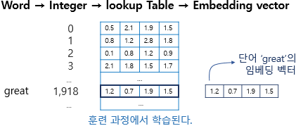
- 자연어 처리의 가장 대표적인 기법 : 워드 임베딩(Word Embedding)
(2) 텍스트 데이터의 특징
- 텍스트는 숫자 행렬로 변환할 필요가 없다.
- 텍스트에는 입력 순서가 중요하다.
(3) 텍스트를 숫자로 표현하는 방법
# 처리해야 할 문장을 파이썬 리스트에 옮기기
sentences=['i am hungry', 'i like apple', 'i am so happy']

# 파이썬 split() 메소드를 이용해 단어 단위로 문장을 쪼개기
word_list = 'i am hungry'.split()
print(word_list)

index_to_word={}  # 빈 딕셔너리를 만들어서

# 단어들을 하나씩 채워보자. 순서는 중요하지 않다.
# <BOS>, <PAD>, <UNK>는 관례적으로 딕셔너리 맨 앞에 넣어준다
index_to_word[0]='<PAD>'  # 패딩용 단어
index_to_word[1]='<BOS>'  # 문장의 시작지점
index_to_word[2]='<UNK>'  # 사전에 없는(Unknown) 단어
index_to_word[3]='i'
index_to_word[4]='like'
index_to_word[5]='hungry'
index_to_word[6]='so'
index_to_word[7]='apple'
index_to_word[8]='happy'

print(index_to_word)

word_to_index={word:index for index, word in index_to_word.items()}
print(word_to_index)

# 문장 1개를 활용할 딕셔너리와 함께 주면, 단어 인덱스 리스트로 변환해 주는 함수
# 단, 모든 문장은 <BOS>로 시작하는 것으로 합니다.
def get_encoded_sentence(sentence, word_to_index):
    return [word_to_index['<BOS>']]+[word_to_index[word] if word in word_to_index else word_to_index['<UNK>'] for word in sentence.split()]

# 여러 개의 문장 리스트를 한꺼번에 숫자 텐서로 encode해 주는 함수
def get_encoded_sentences(sentences, word_to_index):
    return [get_encoded_sentence(sentence, word_to_index) for sentence in sentences]

# 숫자 벡터로 encode된 문장을 원래대로 decode하는 함수
def get_decoded_sentence(encoded_sentence, index_to_word):
    return ' '.join(index_to_word[index] if index in index_to_word else '<UNK>' for index in encoded_sentence[1:])  #[1:]를 통해 <BOS>를 제외

# 여러개의 숫자 벡터로 encode된 문장을 한꺼번에 원래대로 decode하는 함수
def get_decoded_sentences(encoded_sentences, index_to_word):
    return [get_decoded_sentence(encoded_sentence, index_to_word) for encoded_sentence in encoded_sentences]
(4) Embedding 레이어의 등장
# raw_inputs의 문장의 길이를 PAD를 이용하여 동일하게 만들기
raw_inputs = keras.preprocessing.sequence.pad_sequences(raw_inputs,
                                                       value=word_to_index['<PAD>'],
                                                       padding='post',
                                                       maxlen=5)
print(raw_inputs)

# Embedding
import numpy as np
import tensorflow as tf

vocab_size = len(word_to_index)  # 위 예시에서 딕셔너리에 포함된 단어 개수는 10
word_vector_dim = 4    # 그림과 같이 4차원의 워드벡터를 가정

embedding = tf.keras.layers.Embedding(input_dim=vocab_size, output_dim=word_vector_dim, mask_zero=True)

# keras.preprocessing.sequence.pad_sequences를 통해 word vector를 모두 일정길이로 맞춰주어야
# embedding 레이어의 input이 될 수 있음에 주의
raw_inputs = np.array(get_encoded_sentences(sentences, word_to_index))
raw_inputs = keras.preprocessing.sequence.pad_sequences(raw_inputs,
                                                       value=word_to_index['<PAD>'],
                                                       padding='post',
                                                       maxlen=5)
output = embedding(raw_inputs)
print(output)
(5) 시퀀스 데이터를 다루는 RNN(Recurrnet Neural Network)
# RNN 모델을 사용하여 텍스트 데이터 처리
model = keras.Sequential()
model.add(keras.layers.Embedding(vocab_size, word_vector_dim, input_shape=(None,)))
model.add(keras.layers.LSTM(8))   # 가장 널리 쓰이는 RNN인 LSTM 레이어를 사용
model.add(keras.layers.Dense(8, activation='relu'))
model.add(keras.layers.Dense(1, activation='sigmoid'))

model.summary()
텍스트를 처리하기 위해 RNN이 아니라 1-D CNN을 사용할 수도 있다. 텍스트는 시퀀스 데이터이기 때문에 1-D CNN 으로 문장 전체를 한꺼번에 한 방향으로 스캔하여 발견되는 특징을 추출해서 문장을 분류하는 방식으로 사용된다. CNN 계열은 RNN 계열보다 병렬처리가 효율적이기 때문에 학습 속도도 훨씬 빠르게 진행된다는 장점이 있다.
# 1DConv 모델을 사용하여 텍스트 데이터 처리
model = keras.Sequential()
model.add(keras.layers.Embedding(vocab_size, word_vector_dim, input_shape=(None,)))
model.add(keras.layers.Conv1D(16, 7, activation='relu'))
model.add(keras.layers.MaxPooling1D(5))
model.add(keras.layers.Conv1D(16, 7, activation='relu'))
model.add(keras.layers.GlobalMaxPooling1D())
model.add(keras.layers.Dense(8, activation='relu'))
model.add(keras.layers.Dense(1, activation='sigmoid'))

model.summary()
아주 간단히는 GlobalMaxPooling1D() 레이어 하나만 사용하는 방법도 생각할 수 있다. 이 방식은 전체 문장 중 가장 중요한 단 하나의 특징만을 추출해서 문장의 긍정/부정을 평가하는 방식이다.
# GlobalMaxPooling1D 모델을 사용하여 텍스트 데이터 처리
model = keras.Sequential()
model.add(keras.layers.Embedding(vocab_size, word_vector_dim, input_shape=(None,)))
model.add(keras.layers.GlobalMaxPooling1D())
model.add(keras.layers.Dense(8, activation='relu'))
model.add(keras.layers.Dense(1, activation='sigmoid'))

model.summary()
이 외에도 1-D CNN과 RNN을 섞어 쓴다거나, FFN(FeedForword Network) 레이어만으로 구성하거나, Transformer 레이어를 쓰는 등 다양한 시도를 해볼 수 있다.
IMDB 영화리뷰 감성분석
(1) IMDB 데이터셋 분석
IMDB Large Movie Dataset은 50000개의 영어로 작성된 영화 리뷰 텍스트로 구성되어 있으며, 긍정은 1, 부정은 0의 라벨이 달려있다. 이 중 25000개가 훈련용 데이터, 나머지 25000개를 테스트 데이터로 사용하도록 지정되어 있다.
import tensorflow as tf
from tensorflow import keras
import numpy as np

print(tf.__version__)
imdb = keras.datasets.imdb

# IMDB 데이터셋 다운로드
(x_train, y_train), (x_test, y_test) = imdb.load_data(num_words=10000)
print("훈련 샘플 개수: {}, 테스트 개수: {}".format(len(x_train), len(x_test)))

# 데이터 확인
print(x_train[0])  # 1번째 리뷰데이터
print('라벨: ', y_train[0])  # 1번째 리뷰데이터의 라벨
print('1번째 리뷰 문장 길이: ', len(x_train[0]))

# word_index 가져오기
word_to_index = imdb.get_word_index()
index_to_word = {index:word for word, index in word_to_index.items()}
print(index_to_word[1])     # 'the' 가 출력
print(word_to_index['the'])  # 1 이 출력

# decoding
print(get_decoded_sentence(x_train[0], index_to_word))
print('라벨: ', y_train[0])  # 1번째 리뷰데이터의 라벨

# 텍스트데이터 문장길이의 리스트를 생성한 후
total_data_text = list(x_train) + list(x_test)

# 문장길이의 평균값, 최대값, 표준편차를 계산
num_tokens = [len(tokens) for tokens in total_data_text]
num_tokens = np.array(num_tokens)

print('문장길이 평균 : ', np.mean(num_tokens))
print('문장길이 최대 : ', np.max(num_tokens))
print('문장길이 표준편차 : ', np.std(num_tokens))

# 예를들어, 최대 길이를 (평균 + 2*표준편차)로 한다면,
max_tokens = np.mean(num_tokens) + 2 * np.std(num_tokens)
maxlen = int(max_tokens)
print('pad_sequences maxlen : ', maxlen)
print('전체 문장의 {}%가 maxlen 설정값 이내에 포함됩니다. '.format(np.sum(num_tokens < max_tokens) / len(num_tokens)))

# padding
x_train = keras.preprocessing.sequence.pad_sequences(x_train,
                                                        value=word_to_index["<PAD>"],
                                                        padding='post', # 혹은 'pre'
                                                        maxlen=maxlen)

x_test = keras.preprocessing.sequence.pad_sequences(x_test,
                                                       value=word_to_index["<PAD>"],
                                                       padding='post', # 혹은 'pre'
                                                       maxlen=maxlen)

print(x_train.shape)
(2) 딥러닝 모델 설계와 훈련
vocab_size = 10000    # 어휘 사전의 크기입니다(10,000개의 단어)
word_vector_dim = 16  # 워드 벡터의 차원수 (변경가능한 하이퍼파라미터)

# model 설계
model = keras.Sequential()
model.add(keras.layers.Embedding(vocab_size, word_vector_dim, input_shape=(None,)))
model.add(keras.layers.LSTM(8))   # 가장 널리 쓰이는 RNN인 LSTM 레이어를 사용
model.add(keras.layers.Dense(8, activation='relu'))
model.add(keras.layers.Dense(1, activation='sigmoid'))  # 최종 출력은 긍정/부정을 나타내는 1dim

model.summary()

# validation set 10000건 분리
x_val = x_train[:10000]
y_val = y_train[:10000]

# validation set을 제외한 나머지 15000건
partial_x_train = x_train[10000:]
partial_y_train = y_train[10000:]

print(partial_x_train.shape)
print(partial_y_train.shape)

# 모델 학습
model.compile(optimizer='adam',
              loss='binary_crossentropy',
              metrics=['accuracy'])

epochs=20

history = model.fit(partial_x_train,
                    partial_y_train,
                    epochs=epochs,
                    batch_size=512,
                    validation_data=(x_val, y_val),
                    verbose=1)

# 모델 평가
results = model.evaluate(x_test,  y_test, verbose=2)

print(results)

# 모델의 fitting 과정 중의 정보들이 history 변수에 저장
history_dict = history.history
print(history_dict.keys()) # epoch에 따른 그래프를 그려볼 수 있는 항목들

# 도식화 Training and Validation loss
import matplotlib.pyplot as plt

acc = history_dict['accuracy']
val_acc = history_dict['val_accuracy']
loss = history_dict['loss']
val_loss = history_dict['val_loss']

epochs = range(1, len(acc) + 1)

# "bo"는 "파란색 점"입니다
plt.plot(epochs, loss, 'bo', label='Training loss')
# b는 "파란 실선"입니다
plt.plot(epochs, val_loss, 'b', label='Validation loss')
plt.title('Training and validation loss')
plt.xlabel('Epochs')
plt.ylabel('Loss')
plt.legend()

plt.show()

# Training and Validation accuracy
plt.clf()   # 그림을 초기화

plt.plot(epochs, acc, 'bo', label='Training acc')
plt.plot(epochs, val_acc, 'b', label='Validation acc')
plt.title('Training and validation accuracy')
plt.xlabel('Epochs')
plt.ylabel('Accuracy')
plt.legend()

plt.show()
(3) Word2Vec의 적용
pip install gensim : 워드벡터를 다루는데 유용한 패키지
# 임베딩 레이어 생성
embedding_layer = model.layers[0]
weights = embedding_layer.get_weights()[0]
print(weights.shape)    # shape: (vocab_size, embedding_dim)

# 학습한 Embedding 파라미터를 저장
import os

word2vec_file_path = os.getenv('HOME')+'/aiffel/sentiment_classification/word2vec.txt'
f = open(word2vec_file_path, 'w')
f.write('{} {}\n'.format(vocab_size-4, word_vector_dim))  # 몇개의 벡터를 얼마 사이즈로 기재할지

# 단어 개수(에서 특수문자 4개는 제외하고)만큼의 워드 벡터를 파일에 기록
vectors = model.get_weights()[0]
for i in range(4,vocab_size):
    f.write('{} {}\n'.format(index_to_word[i], ' '.join(map(str, list(vectors[i, :])))))
f.close()

# gensim 에서 제공하는 패키지를 이용하여 임베딩 파라미터를 word vector로 사용
from gensim.models.keyedvectors import Word2VecKeyedVectors

word_vectors = Word2VecKeyedVectors.load_word2vec_format(word2vec_file_path, binary=False)
vector = word_vectors['computer']
vector

# 단어 유사도 분석
word_vectors.similar_by_word("love")
감성분류 태스크를 잠깐 학습한 것 만으로는 워드벡터가 유의미하게 학습되기 어려운 것 같다. 이 정도의 훈련 데이터로는 워드벡터를 정교하게 학습시키기 어렵다고 한다. 따라서 구글에서 제공하는 Word2Vec라는 사전 학습된 워드 임베딩 모델을 활용해보자. 다운로드
# 모델 불러오기
from gensim.models import KeyedVectors
word2vec_path = os.getenv('HOME')+'/aiffel/sentiment_classification/GoogleNews-vectors-negative300.bin.gz'
word2vec = KeyedVectors.load_word2vec_format(word2vec_path, binary=True, limit=None)
vector = word2vec['computer']
vector     # 300dim의 워드 벡터. limit으로 조건을 주어 로딩 가능

# 단어 유사도 분석
word2vec.similar_by_word("love")

# 임베딩 레이어 변경
vocab_size = 10000    # 어휘 사전의 크기입니다(10,000개의 단어)
word_vector_dim = 300  # 워드 벡터의 차원수 (변경가능한 하이퍼파라미터)

embedding_matrix = np.random.rand(vocab_size, word_vector_dim)

# embedding_matrix에 Word2Vec 워드벡터를 단어 하나씩마다 차례차례 카피
for i in range(4,vocab_size):
    if index_to_word[i] in word2vec:
        embedding_matrix[i] = word2vec[index_to_word[i]]

# 모델 설계
from tensorflow.keras.initializers import Constant

vocab_size = 10000    # 어휘 사전의 크기입니다(10,000개의 단어)
word_vector_dim = 300  # 워드 벡터의 차원수 (변경가능한 하이퍼파라미터)

# 모델 구성
model = keras.Sequential()
model.add(keras.layers.Embedding(vocab_size,
                                 word_vector_dim,
                                 embeddings_initializer=Constant(embedding_matrix),  # 카피한 임베딩을 여기서 활용
                                 input_length=maxlen,
                                 trainable=True))   # trainable을 True로 주면 Fine-tuning
model.add(keras.layers.Conv1D(16, 7, activation='relu'))
model.add(keras.layers.MaxPooling1D(5))
model.add(keras.layers.Conv1D(16, 7, activation='relu'))
model.add(keras.layers.GlobalMaxPooling1D())
model.add(keras.layers.Dense(8, activation='relu'))
model.add(keras.layers.Dense(1, activation='sigmoid'))

model.summary()

# 모델 학습
model.compile(optimizer='adam',
              loss='binary_crossentropy',
              metrics=['accuracy'])

epochs=20

history = model.fit(partial_x_train,
                    partial_y_train,
                    epochs=epochs,
                    batch_size=512,
                    validation_data=(x_val, y_val),
                    verbose=1)

# 모델 평가
results = model.evaluate(x_test,  y_test, verbose=2)

print(results)이버 영화리뷰 감성분석 도전하기
(1) 데이터 준비와 확인
import pandas as pd
import urllib.request
%matplotlib inline
import matplotlib.pyplot as plt
import re
from konlpy.tag import Okt
from tensorflow import keras
from tensorflow.keras.preprocessing.text import Tokenizer
import numpy as np
from tensorflow.keras.preprocessing.sequence import pad_sequences
from collections import Counter
import os

# 데이터 읽기
train_data = pd.read_table('~/aiffel/sentiment_classification/ratings_train.txt')
test_data = pd.read_table('~/aiffel/sentiment_classification/ratings_test.txt')

train_data.head()
(2) 데이터 로더 구성
data_loader를 직접 만들어보자. data_loader에서는 다음을 수행해야 한다.
- 데이터의 중복 제거
- NaN 결측치 제거
- 한국어 토크나이저로 토큰화
- 불용어(Stopwords) 제거
- 사전word_to_index 구성
- 텍스트 스트링을 사전 인덱스 스트링으로 변환
- X_train, y_train, X_test, y_test, word_to_index 리턴
from konlpy.tag import Mecab
tokenizer = Mecab()
stopwords = ['의','가','이','은','들','는','좀','잘','걍','과','도','를','으로','자','에','와','한','하다']

# load_data 함수
def load_data(train_data, test_data, num_words=10000):
    train_data.drop_duplicates(subset=['document'], inplace=True)
    train_data = train_data.dropna(how = 'any')
    test_data.drop_duplicates(subset=['document'], inplace=True)
    test_data = test_data.dropna(how = 'any')

    x_train = []
    for sentence in train_data['document']:
        temp_x = tokenizer.morphs(sentence) # 토큰화
        temp_x = [word for word in temp_x if word not in stopwords] # 불용어 제거
        x_train.append(temp_x)

    x_test = []
    for sentence in test_data['document']:
        temp_x = tokenizer.morphs(sentence) # 토큰화
        temp_x = [word for word in temp_x if word not in stopwords] # 불용어 제거
        x_test.append(temp_x)

    words = np.concatenate(x_train).tolist()
    counter = Counter(words)
    counter = counter.most_common(10000-4)
    vocab = ['<PAD>', '<BOS>', '<UNK>', '<UNUSED>'] + [key for key, _ in counter]
    word_to_index = {word:index for index, word in enumerate(vocab)}

    def wordlist_to_indexlist(wordlist):
        return [word_to_index[word] if word in word_to_index else word_to_index['<UNK>'] for word in wordlist]

    x_train = list(map(wordlist_to_indexlist, x_train))
    x_test = list(map(wordlist_to_indexlist, x_test))

    return x_train, np.array(list(train_data['label'])), x_test, np.array(list(test_data['label'])), word_to_index

x_train, y_train, x_test, y_test, word_to_index = load_data(train_data, test_data)

index_to_word = {index:word for word, index in word_to_index.items()}

# 문장 1개를 활용할 딕셔너리와 함께 주면, 단어 인덱스 리스트 벡터로 변환해 주는 함수
# 단, 모든 문장은 <BOS>로 시작
def get_encoded_sentence(sentence, word_to_index):
    return [word_to_index['<BOS>']]+[word_to_index[word] if word in word_to_index else word_to_index['<UNK>'] for word in sentence.split()]

# 여러 개의 문장 리스트를 한꺼번에 단어 인덱스 리스트 벡터로 encode해 주는 함수
def get_encoded_sentences(sentences, word_to_index):
    return [get_encoded_sentence(sentence, word_to_index) for sentence in sentences]

# 숫자 벡터로 encode된 문장을 원래대로 decode하는 함수
def get_decoded_sentence(encoded_sentence, index_to_word):
    return ' '.join(index_to_word[index] if index in index_to_word else '<UNK>' for index in encoded_sentence[1:])  #[1:]를 통해 <BOS>를 제외

# 여러개의 숫자 벡터로 encode된 문장을 한꺼번에 원래대로 decode하는 함수
def get_decoded_sentences(encoded_sentences, index_to_word):
    return [get_decoded_sentence(encoded_sentence, index_to_word) for encoded_sentence in encoded_sentences]

print("훈련 샘플 개수: {}, 테스트 개수: {}".format(len(x_train), len(x_test)))

# decoding
print(get_decoded_sentence(x_train[0], index_to_word))
print('라벨: ', y_train[0])  # 1번째 리뷰데이터의 라벨

# 텍스트데이터 문장길이의 리스트를 생성한 후
total_data_text = list(x_train) + list(x_test)

# 문장길이의 평균값, 최대값, 표준편차를 계산
num_tokens = [len(tokens) for tokens in total_data_text]
num_tokens = np.array(num_tokens)

print('문장길이 평균 : ', np.mean(num_tokens))
print('문장길이 최대 : ', np.max(num_tokens))
print('문장길이 표준편차 : ', np.std(num_tokens))
plt.clf()

plt.hist([len(s) for s in total_data_text], bins=100)
plt.xlabel('length of samples')
plt.ylabel('number of samples')
plt.show()

# 예를들어, 최대 길이를 (평균 + 2*표준편차)로 가정
max_tokens = np.mean(num_tokens) + 2 * np.std(num_tokens)
maxlen = int(max_tokens)
print('pad_sequences maxlen : ', maxlen)
print('전체 문장의 {}%가 maxlen 설정값 이내에 포함됩니다. '.format(np.sum(num_tokens < max_tokens) / len(num_tokens)))

# padding
x_train = keras.preprocessing.sequence.pad_sequences(x_train,
                                                        value=word_to_index["<PAD>"],
                                                        padding='pre', # 혹은 'pre'
                                                        maxlen=maxlen)

x_test = keras.preprocessing.sequence.pad_sequences(x_test,
                                                       value=word_to_index["<PAD>"],
                                                       padding='pre', # 혹은 'pre'
                                                       maxlen=maxlen)

print(x_train.shape)

vocab_size = 10000    # 어휘 사전의 크기입니다(10,000개의 단어)
word_vector_dim = 32  # 워드 벡터의 차원수 (변경가능한 하이퍼파라미터)

# 모델 설계
model = keras.Sequential()
model.add(keras.layers.Embedding(vocab_size, word_vector_dim, input_shape=(None,)))
model.add(keras.layers.LSTM(16))
model.add(keras.layers.Dense(8, activation='relu'))
model.add(keras.layers.Dense(1, activation='sigmoid'))

model.summary()

# validation set 10000건 분리
x_val = x_train[:10000]
y_val = y_train[:10000]

# validation set을 제외한 나머지 15000건
partial_x_train = x_train[10000:]
partial_y_train = y_train[10000:]

print(partial_x_train.shape)
print(partial_y_train.shape)

# 모델 학습
model.compile(optimizer='adam',
              loss='binary_crossentropy',
              metrics=['accuracy'])

epochs=10

history = model.fit(partial_x_train,
                    partial_y_train,
                    epochs=epochs,
                    batch_size=512,
                    validation_data=(x_val, y_val),
                    verbose=1)

# 모델 평가
results = model.evaluate(x_test,  y_test, verbose=2)

print(results)

# 모델의 fitting 과정 중의 정보들이 history 변수에 저장
history_dict = history.history
print(history_dict.keys()) # epoch에 따른 그래프를 그려볼 수 있는 항목들

acc = history_dict['accuracy']
val_acc = history_dict['val_accuracy']
loss = history_dict['loss']
val_loss = history_dict['val_loss']

epochs = range(1, len(acc) + 1)

# "bo"는 "파란색 점"
plt.plot(epochs, loss, 'bo', label='Training loss')
# b는 "파란 실선"
plt.plot(epochs, val_loss, 'b', label='Validation loss')
plt.title('Training and validation loss')
plt.xlabel('Epochs')
plt.ylabel('Loss')
plt.legend()

plt.show()

# Training and Validation accuracy
plt.clf()   # 그림을 초기화

plt.plot(epochs, acc, 'bo', label='Training acc')
plt.plot(epochs, val_acc, 'b', label='Validation acc')
plt.title('Training and validation accuracy')
plt.xlabel('Epochs')
plt.ylabel('Accuracy')
plt.legend()

plt.show()
(3) gensim을 이용하여 사전학습 된 모델 이용하기
Pre-trained된 Word2Vec Embedding을 이용하여 정확도를 올려보자.
import gensim
word2vec_path = os.getenv('HOME')+'/aiffel/sentiment_classification/ko.bin'
pre_word2vec = gensim.models.Word2Vec.load(word2vec_path)
vector = pre_word2vec.wv.most_similar("강아지")
vector

pre_word2vec['강아지'].shape

# 임베딩 레이어 변경
vocab_size = 10000    # 어휘 사전의 크기입니다(10,000개의 단어)
word_vector_dim = 200  # 워드 벡터의 차원수 (변경가능한 하이퍼파라미터)

embedding_matrix = np.random.rand(vocab_size, word_vector_dim)

# embedding_matrix에 Word2Vec 워드벡터를 단어 하나씩마다 차례차례 카피
for i in range(4,vocab_size):
    if index_to_word[i] in pre_word2vec:
        embedding_matrix[i] = pre_word2vec[index_to_word[i]]

# 모델 설계
from tensorflow.keras.initializers import Constant

vocab_size = 10000    # 어휘 사전의 크기입니다(10,000개의 단어)
word_vector_dim = 200  # 워드 벡터의 차원수 (변경가능한 하이퍼파라미터)

# 모델 구성
model = keras.Sequential()
model.add(keras.layers.Embedding(vocab_size,
                                 word_vector_dim,
                                 embeddings_initializer=Constant(embedding_matrix),  # 카피한 임베딩을 여기서 활용
                                 input_length=maxlen,
                                 trainable=True))   # trainable을 True로 주면 Fine-tuning
model.add(keras.layers.LSTM(16))
model.add(keras.layers.Dense(8, activation='relu'))
model.add(keras.layers.Dense(1, activation='sigmoid'))

model.summary()

# 모델 학습
model.compile(optimizer='adam',
              loss='binary_crossentropy',
              metrics=['accuracy'])

epochs=15

history = model.fit(partial_x_train,
                    partial_y_train,
                    epochs=epochs,
                    batch_size=4096,
                    validation_data=(x_val, y_val),
                    verbose=1)

# 모델 평가
results = model.evaluate(x_test,  y_test, verbose=2)

print(results)

# 모델의 fitting 과정 중의 정보들이 history 변수에 저장
history_dict = history.history
print(history_dict.keys()) # epoch에 따른 그래프를 그려볼 수 있는 항목들

# 도식화 Training and Validation loss
import matplotlib.pyplot as plt

acc = history_dict['accuracy']
val_acc = history_dict['val_accuracy']
loss = history_dict['loss']
val_loss = history_dict['val_loss']

epochs = range(1, len(acc) + 1)

# "bo"는 "파란색 점"입니다
plt.plot(epochs, loss, 'bo', label='Training loss')
# b는 "파란 실선"입니다
plt.plot(epochs, val_loss, 'b', label='Validation loss')
plt.title('Training and validation loss')
plt.xlabel('Epochs')
plt.ylabel('Loss')
plt.legend()

plt.show()

# Training and Validation accuracy
plt.clf()   # 그림을 초기화합니다

plt.plot(epochs, acc, 'bo', label='Training acc')
plt.plot(epochs, val_acc, 'b', label='Validation acc')
plt.title('Training and validation accuracy')
plt.xlabel('Epochs')
plt.ylabel('Accuracy')
plt.legend()

plt.show()
회고록
- stateful과 stateless에 대해 몰랐을 땐 손님이 계속 이전의 선택지를 이야기 해주기 때문에 손님이 state를 결정한다고 생각했는데 직원이 기억하지 못하여 손님이 선택지를 이야기해주는 것이어서 state를 결정하는 것은 직원이었다.
- RNN 활용 시 pad_sequences의 padding 방식은 post와 pre중 post가 추후 0으로 padding된 부분의 연산을 수행하지 않아도 될 것 같아서 post 방식이 유리할 것으로 예상했지만, 실제로는 RNN의 가장 마지막 입력이 최종 state 값에 가장 영향을 많이 미치기 때문에 마지막 입력이 무의미한 padding으로 채워지는 것은 비효율 적이라고 한다. 따라서 pre가 훨씬 유리하며 10% 이상의 테스트 성능 차이를 보인다고 한다.
- 정확도를 85%로 올리기 위해 LSTM, 1-D Conv, GlobalMaxPooling 등 다양한 모델에서 각종 Hyperparameter를 이것저것 변화시켜 보았지만 85%는 넘을 수가 없었다. 결국 Word2Vec를 이용하여 Pre-Trained된 Word2Vec Embedding 모델을 사용하였지만 이 모델에서도 유일하게 LSTM 만 85%를 아슬아슬하게 넘을 수 있었다.
- 아직 머신러닝이나 딥러닝의 모델을 설계하는 정확한 이해 없이 정확도를 올리려고 하니까 너무 어려운 것 같다. 물론 아직 배우기 시작하는 단계라서 어쩔 수 없다고 생각은 하지만 모델 설계에 대한 공부도 따로 해야겠다.
- 일단 이미지 인식과 자연어 처리 둘 다 경험은 해봤으니 앞으로 어떤 분야에 집중을 할지 고민해봐야겠다.
유용한 링크
https://dbr.donga.com/article/view/1202/article_no/8891/ac/magazine
https://ratsgo.github.io/natural language processing/2019/09/12/embedding/ 한국어 임베딩
'AIFFEL' 카테고리의 다른 글
| [SSAC X AIFFEL] 작사가 인공지능 만들기 (0) | 2021.02.08 |
|---|---|
| [SSAC X AIFFEL] 인공지능 모델로 음성 단어 구분하기 (1) | 2021.01.29 |
| [SSAC X AIFFEL] 카메라 스티커 앱 만들기 첫걸음 (2) | 2021.01.13 |
| [SSAC X AIFFEL] 사이킷런(scikit-learn): Iris 품종 분류해보기 (0) | 2021.01.08 |
| [SSAC X AIFFEL] 첫 딥러닝 모델: 가위바위보 분류기 (0) | 2021.01.05 |