오늘은 아이펠 첫 Exploration 노드를 진행하였다. 나는 이론보다는 실전파라 더 기대가 되는 날이었다. 매번 인터넷으로만 보던 딥러닝 모델을 내가 직접 구현해볼 수 있는 아주 좋은 기회였다. 물론 처음부터 모든 코드를 내가 짠 것은 아니지만, 지금은 어떻게 작동을 하는지 그 원리를 이해하고 익히는 것이 중요하다고 생각한다. 처음에는 노드를 열심히 따라가면서 코드를 하나하나 실행시켜 보는 것으로 시작해서, 가위바위보를 분류하는 모델은 앞서 모델링되어있는 자료를 참고하여 내가 직접 복붙(?)한 코드이다. 물론 MNIST를 이용한 숫자 분류와는 조금 다른 부분이 있어서 해당 부분만 수정할 줄 안다면 그다지 어렵지 않은 과제였다. 라고 생각했던 때가 있었지...
How to make?
일반적으로 딥러닝 기술은 "데이터 준비 → 딥러닝 네트워크 설계 → 학습 → 테스트(평가)" 순으로 이루어진다.
1. 데이터 준비
MINIST 숫자 손글씨 Dataset 불러들이기
import tensorflow as tf
from tensorflow import keras

import numpy as np
import matplotlib.pyplot as plt

print(tf.__version__) # Tensorflow의 버전 출력

mnist = keras.datasets.mnist

(x_train, y_train), (x_test, y_test) = mnist.load_data()

print(len(x_train)) # x_train 배열의 크기를 출력

plt.imshow(x_train[1], cmap=plt.cm.binary)
plt.show() # x_train의 1번째 이미지를 출력

print(y_train[1]) # x_train[1]에 대응하는 실제 숫자값

index = 10000
plt.imshow(x_train[index], cmap=plt.cm.binary)
plt.show()
print(f'{index} 번째 이미지의 숫자는 바로 {y_train[index]} 입니다.')

print(x_train.shape) # x_train 이미지의 (count, x, y)
print(x_test.shape)
Data 전처리 하기
인공지능 모델을 훈련시킬 때, 값이 너무 커지거나 하는 것을 방지하기 위해 정수 연산보다는 0~1 사이의 값으로 정규화 시켜주는 것이 좋다.
정규화는 모든 값을 최댓값으로 나누어주면 된다.
print(f'최소값: {np.min(x_train)} 최대값: {np.max(x_train)}')

x_train_norm, x_test_norm = x_train / 255.0, x_test / 255.0
print(f'최소값: {np.min(x_train_norm)} 최대값: {np.max(x_train_norm)}')
2. 딥러닝 네트워크 설계하기
Sequential Model 사용해보기
model = keras.models.Sequential()
model.add(keras.layers.Conv2D(16, (3,3), activation='relu', input_shape=(28,28,1)))
model.add(keras.layers.MaxPool2D(2,2))
model.add(keras.layers.Conv2D(32, (3,3), activation='relu'))
model.add(keras.layers.MaxPooling2D((2,2)))
model.add(keras.layers.Flatten())
model.add(keras.layers.Dense(32, activation='relu'))
model.add(keras.layers.Dense(10, activation='softmax'))

print(f'Model에 추가된 Layer 개수: {len(model.layers)}')

model.summary()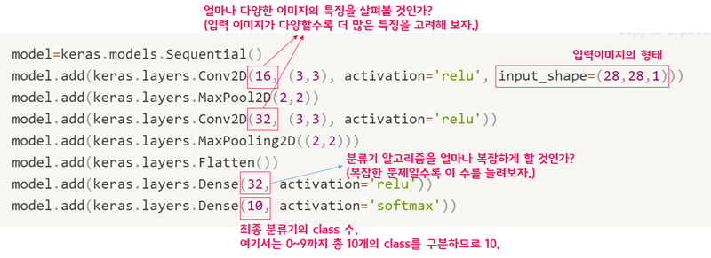
3. 딥러닝 네트워크 학습시키기
우리가 만든 네트워크의 입력은 (data_size, x_size, y_size, channel) 과 같은 형태를 가진다. 그러나 x_train.shape 에는 채널수에 대한 정보가 없기 때문에 만들어주어야 한다.
print("Before Reshape - x_train_norm shape: {}".format(x_train_norm.shape))
print("Before Reshape - x_test_norm shape: {}".format(x_test_norm.shape))

x_train_reshaped=x_train_norm.reshape( -1, 28, 28, 1)  # 데이터갯수에 -1을 쓰면 reshape시 자동계산됩니다.
x_test_reshaped=x_test_norm.reshape( -1, 28, 28, 1)

print("After Reshape - x_train_reshaped shape: {}".format(x_train_reshaped.shape))
print("After Reshape - x_test_reshaped shape: {}".format(x_test_reshaped.shape))

model.compile(optimizer='adam',
             loss='sparse_categorical_crossentropy',
             metrics=['accuracy'])

model.fit(x_train_reshaped, y_train, epochs=10)
10epochs 정도 돌려본 결과 99.8% 에 가까운 정확도를 나타내는 것을 확인하였다.
4. 모델 평가하기
테스트 데이터로 성능을 확인해보기
test_loss, test_accuracy = model.evaluate(x_test_reshaped,y_test, verbose=2)
print("test_loss: {} ".format(test_loss))
print("test_accuracy: {}".format(test_accuracy))
실제 테스트 데이터를 이용하여 테스트를 진행해본 결과, 99.1% 로 소폭 하락하였다. MNIST 데이터셋 참고문헌을 보면 학습용 데이터와 시험용 데이터의 손글씨 주인이 다른 것을 알 수 있다.
어떤 데이터를 잘못 추론했는지 확인해보기
model.evalutate() 대신 model.predict()를 사용하면 model이 입력값을 보고 실제로 추론한 확률분포를 출력할 수 있다.
predicted_result = model.predict(x_test_reshaped)  # model이 추론한 확률값.
predicted_labels = np.argmax(predicted_result, axis=1)

idx = 0  # 1번째 x_test를 살펴보자.
print('model.predict() 결과 : ', predicted_result[idx])
print('model이 추론한 가장 가능성이 높은 결과 : ', predicted_labels[idx])
print('실제 데이터의 라벨 : ', y_test[idx])

# 실제 데이터 확인
plt.imshow(x_test[idx],cmap=plt.cm.binary)
plt.show()
추론 결과는 벡터 형태로, 추론 결과가 각각 0, 1, 2, ..., 7, 8, 9 일 확률을 의미한다.
아래 코드는 추론해낸 숫자와 실제 값이 다른 경우를 확인해보는 코드이다.
import random
wrong_predict_list=[]
for i, _ in enumerate(predicted_labels):
    # i번째 test_labels과 y_test이 다른 경우만 모아 봅시다.
    if predicted_labels[i] != y_test[i]:
        wrong_predict_list.append(i)

# wrong_predict_list 에서 랜덤하게 5개만 뽑아봅시다.
samples = random.choices(population=wrong_predict_list, k=5)

for n in samples:
    print("예측확률분포: " + str(predicted_result[n]))
    print("라벨: " + str(y_test[n]) + ", 예측결과: " + str(predicted_labels[n]))
    plt.imshow(x_test[n], cmap=plt.cm.binary)
    plt.show()
5. 더 좋은 네트워크 만들어 보기
딥러닝 네트워크 구조 자체는 바꾸지 않으면서도 인식률을 올릴 수 있는 방법은 Hyperparameter 들을 바꿔보는 것이다. Conv2D 레이어에서 입력 이미지의 특징 수를 증감시켜보거나, Dense 레이어에서 뉴런 수를 바꾸어보거나, epoch 값을 변경해볼 수 있다.
| Title | n_channel_1 | n_channel_2 | n_dense | n_train_epoch | loss | accuracy |
|---|---|---|---|---|---|---|
| 1 | 16 | 32 | 32 | 10 | 0.0417 | 0.9889 |
| 2 | 1 | 32 | 32 | 10 | 0.0636 | 0.9793 |
| 3 | 2 | 32 | 32 | 10 | 0.0420 | 0.9865 |
| 4 | 4 | 32 | 32 | 10 | 0.0405 | 0.9886 |
| 5 | 8 | 32 | 32 | 10 | 0.0360 | 0.9885 |
| 6 | 32 | 32 | 32 | 10 | 0.0322 | 0.9903 |
| 7 | 64 | 32 | 32 | 10 | 0.0325 | 0.9914 |
| 8 | 128 | 32 | 32 | 10 | 0.0320 | 0.9912 |
| 9 | 16 | 1 | 32 | 10 | 0.1800 | 0.9437 |
| 10 | 16 | 64 | 32 | 10 | 0.0322 | 0.9912 |
| 11 | 16 | 128 | 32 | 10 | 0.0348 | 0.9917 |
| 12 | 16 | 32 | 64 | 10 | 0.0430 | 0.9888 |
| 13 | 16 | 32 | 128 | 10 | 0.0327 | 0.9916 |
| 14 | 16 | 32 | 32 | 15 | 0.0427 | 0.9900 |
| 15 | 16 | 32 | 32 | 20 | 0.0523 | 0.9884 |
| 16 | 64 | 128 | 128 | 15 | 0.0503 | 0.9901 |
각각의 Hyperparameter 별로 최적의 값을 찾아서 해당 값들만으로 테스트해보면 가장 좋은 결과가 나올 것 이라고 예상했는데 현실은 아니었다. 이래서 딥러닝이 어려운 것 같다.
6. 프로젝트: 가위바위보 분류기 만들기
오늘 배운 내용을 바탕으로 가위바위보 분류기를 만들어보자.
데이터 준비
1. 데이터 만들기
데이터는 구글의 teachable machine 사이트를 이용하면 쉽게 만들어볼 수 있다.
- 여러 각도에서
- 여러 크기로
- 다른 사람과 함께
- 만들면 더 좋은 데이터를 얻을 수 있다.
다운받은 이미지의 크기는 224x224 이다.
2. 데이터 불러오기 + Resize 하기
MNIST 데이터셋의 경우 이미지 크기가 28x28이었기 때문에 우리의 이미지도 28x28 로 만들어야 한다. 이미지를 Resize 하기 위해 PIL 라이브러리를 사용한다.
# PIL 라이브러리가 설치되어 있지 않다면 설치
!pip install pillow

from PIL import Image
import os, glob

print("PIL 라이브러리 import 완료!")

# 이미지 Resize 하기
# 가위 이미지가 저장된 디렉토리 아래의 모든 jpg 파일을 읽어들여서
image_dir_path = os.getenv("HOME") + "/aiffel/rock_scissor_paper/train/scissor"
print("이미지 디렉토리 경로: ", image_dir_path)

images=glob.glob(image_dir_path + "/*.jpg")

# 파일마다 모두 28x28 사이즈로 바꾸어 저장
target_size=(28,28)
for img in images:
    old_img=Image.open(img)
    new_img=old_img.resize(target_size,Image.ANTIALIAS)
    new_img.save(img,"JPEG")

print("가위 이미지 resize 완료!")
# load_data 함수
def load_data(img_path, number):
# 가위 : 0, 바위 : 1, 보 : 2
number_of_data=number # 가위바위보 이미지 개수 총합
img_size=28
color=3
#이미지 데이터와 라벨(가위 : 0, 바위 : 1, 보 : 2) 데이터를 담을 행렬(matrix) 영역을 생성
imgs=np.zeros(number_of_data*img_size*img_size*color,dtype=np.int32).reshape(number_of_data,img_size,img_size,color)
labels=np.zeros(number_of_data,dtype=np.int32)
idx=0
for file in glob.iglob(img_path+'/scissor/*.jpg'):
img = np.array(Image.open(file),dtype=np.int32)
imgs[idx,:,:,:]=img # 데이터 영역에 이미지 행렬을 복사
labels[idx]=0 # 가위 : 0
idx=idx+1
for file in glob.iglob(img_path+'/rock/*.jpg'):
img = np.array(Image.open(file),dtype=np.int32)
imgs[idx,:,:,:]=img # 데이터 영역에 이미지 행렬을 복사
labels[idx]=1 # 바위 : 1
idx=idx+1
for file in glob.iglob(img_path+'/paper/*.jpg'):
img = np.array(Image.open(file),dtype=np.int32)
imgs[idx,:,:,:]=img # 데이터 영역에 이미지 행렬을 복사
labels[idx]=2 # 보 : 2
idx=idx+1
print("학습데이터(x_train)의 이미지 개수는",idx,"입니다.")
return imgs, labels
image_dir_path = os.getenv("HOME") + "/aiffel/rock_scissor_paper"
(x_train, y_train)=load_data(image_dir_path, 2100)
x_train_norm = x_train/255.0 # 입력은 0~1 사이의 값으로 정규화
print("x_train shape: {}".format(x_train.shape))
print("y_train shape: {}".format(y_train.shape))
# 불러온 이미지 확인
import matplotlib.pyplot as plt
plt.imshow(x_train[0])
print('라벨: ', y_train[0])
# 딥러닝 네트워크 설계
import tensorflow as tf
from tensorflow import keras
import numpy as np
n_channel_1=16
n_channel_2=32
n_dense=64
n_train_epoch=15
model=keras.models.Sequential()
model.add(keras.layers.Conv2D(n_channel_1, (3,3), activation='relu', input_shape=(28,28,3)))
model.add(keras.layers.MaxPool2D(2,2))
model.add(keras.layers.Conv2D(n_channel_2, (3,3), activation='relu'))
model.add(keras.layers.MaxPooling2D((2,2)))
model.add(keras.layers.Flatten())
model.add(keras.layers.Dense(n_dense, activation='relu'))
model.add(keras.layers.Dense(3, activation='softmax'))
model.summary()
# 모델 학습
model.compile(optimizer='adam',
loss='sparse_categorical_crossentropy',
metrics=['accuracy'])
model.fit(x_train_reshaped, y_train, epochs=n_train_epoch)
# 테스트 이미지
image_dir_path = os.getenv("HOME") + "/aiffel/rock_scissor_paper/test/testset1"
(x_test, y_test)=load_data(image_dir_path, 300)
x_test_norm = x_test/255.0 # 입력은 0~1 사이의 값으로 정규화
print("x_train shape: {}".format(x_test.shape))
print("y_train shape: {}".format(y_test.shape))
# 불러온 이미지 확인
import matplotlib.pyplot as plt
plt.imshow(x_test[0])
print('라벨: ', y_test[0])
# 모델 테스트
test_loss, test_accuracy = model.evaluate(x_test_reshaped, y_test, verbose=2)
print("test_loss: {} ".format(test_loss))
print("test_accuracy: {}".format(test_accuracy))처음 100개의 데이터 가지고 실행했을 때 결과는 처참했다...
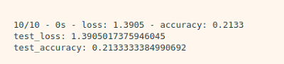
총 10명 분량을 train set으로 사용하고 test를 돌렸을 때 가장 잘 나온 결과!

오늘은 Layer를 추가하지 않고 단순히 Hyperparameter만 조정하여 인식률을 높이는 것을 목표로 했다. 우선 데이터가 부족한 것 같아서 10명 보다 더 많은 데이터를 추가해보면 좋을 것 같다. 아직 첫 모델이라 많이 부족했지만, 그래도 뭔가 목표가 있고 무엇을 해야 하는지 알게 되면 딥러닝이 조금 더 재밌어질 것 같다.
'AIFFEL' 카테고리의 다른 글
| [SSAC X AIFFEL] 인공지능 모델로 음성 단어 구분하기 (1) | 2021.01.29 |
|---|---|
| [SSAC X AIFFEL] 영화리뷰 텍스트 감성분석 하기 (0) | 2021.01.22 |
| [SSAC X AIFFEL] 카메라 스티커 앱 만들기 첫걸음 (2) | 2021.01.13 |
| [SSAC X AIFFEL] 사이킷런(scikit-learn): Iris 품종 분류해보기 (0) | 2021.01.08 |
| [SSAC X AIFFEL] 첫 글쓰기 (0) | 2020.12.31 |